Unveiling The Structure of Hierarchical Time Series
Hierarchical Time Series
Real forecasting tasks typically involve a large number of time series. Think of the relevant time series to electricity generation in the US: total generated per state/region, per fuel source, per ultimate customer (industrial or residential). All of these series are related: the state-level generation adds up to the regional generation, which should add up to the national total. This structured collection of time series, connected by aggregation rules, is what we call Hierarchical Time Series.
Hierarchical time series appear everywhere: finance (portfolio → sector → asset), retail (company → region → store → product), energy (country → region → substation), and operations (organization → department → team). The hierarchy encodes how finer-grained series roll up into higher-level summaries, and that structure is both a constraint and an opportunity for better forecasting.
In order to define mathematically a hierarchical system we need to notice that all time series in the hierarchy are defined as sums of some the bottom level series (most disaggregated).
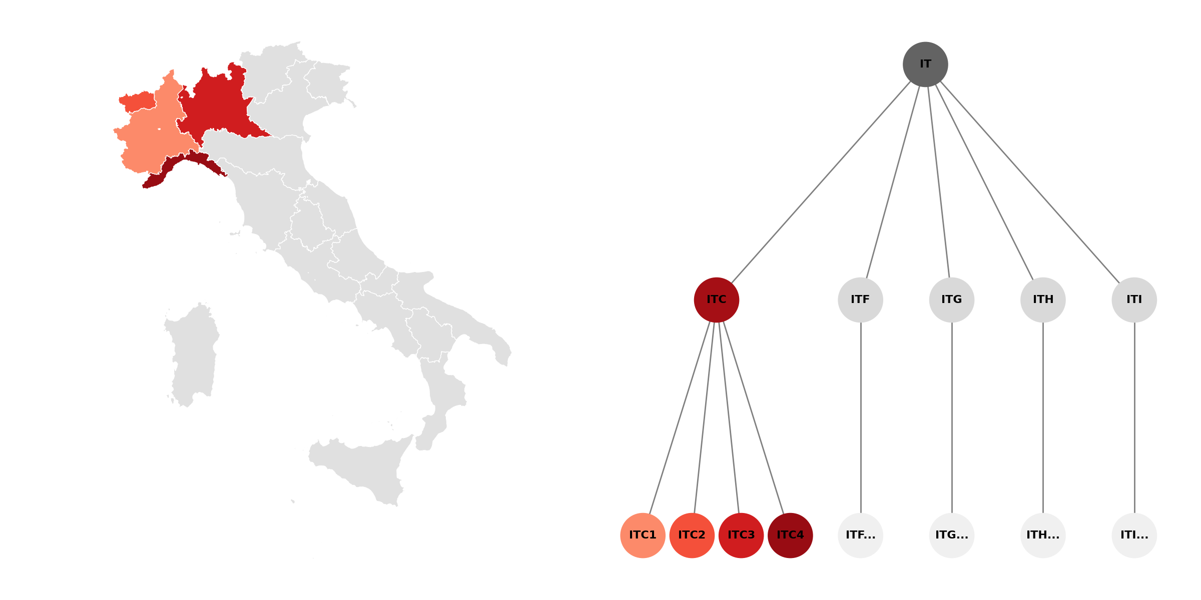
Thus given $\mathbf{y}_t \in \mathbb{R}^n$ the vector of all time series and $\mathbf{b}_t \in \mathbb{R}^m$ the vector of bottom time series (note $m<n$). The hierarchy is fully defined by the summing matrix $S$ s.t.
\[\begin{align} \mathbf{y}_t = S \mathbf{b}_t \;\;\;\;\;\;\;\;\;\;\;\;\;\;\;\;\;\;\; \|\mathbf{y}_t - S\mathbf{b}_t\| = \mathrm{C}_t = 0 \end{align}\]Note : Forecasts are not always coherent ($\mathrm{C}_t \neq 0$). $\mathrm{C}_t$ measures the incoherence or the distance from the hierarchical structure for each possible set of values
\[\underbrace{ \begin{bmatrix} \mathrm{IT}_t \\[2pt] \color{red}{\mathrm{ITC}_t} \\[2pt] \mathrm{ITF}_t \\[2pt] \mathrm{ITG}_t \\[2pt] \mathrm{ITH}_t \\[2pt] \mathrm{ITI}_t \\[4pt] \color{salmon}{\mathrm{ITC1}_t} \\[2pt] \color{coral}{\mathrm{ITC2}_t} \\[2pt] \color{crimson}{\mathrm{ITC3}_t} \\[2pt] \color{maroon}{\mathrm{ITC4}_t} \\[2pt] \vdots \end{bmatrix} }_{\mathbf{y}_t} = \underbrace{ \begin{bmatrix} 1 & 1 & 1 & 1 & 1 & \cdots & 1 & \cdots \\[4pt] \color{red}{1} & \color{red}{1} & \color{red}{1} & \color{red}{1} & 0 & \cdots & 0 & \cdots \\[4pt] 0 & 0 & 0 & 0 & 1 & \cdots & 1 & \cdots \\[4pt] 0 & 0 & 0 & 0 & 0 & \cdots & 0 & \cdots \\[4pt] 0 & 0 & 0 & 0 & 0 & \cdots & 0 & \cdots \\[4pt] 0 & 0 & 0 & 0 & 0 & \cdots & 0 & \cdots \\[4pt] \hline \color{salmon}{1} & 0 & 0 & 0 & 0 & \cdots & 0 & \cdots \\[2pt] 0 & \color{coral}{1} & 0 & 0 & 0 & \cdots & 0 & \cdots \\[2pt] 0 & 0 & \color{crimson}{1} & 0 & 0 & \cdots & 0 & \cdots \\[2pt] 0 & 0 & 0 & \color{maroon}{1} & 0 & \cdots & 0 & \cdots \\[2pt] 0 & 0 & 0 & 0 & 1 & \cdots & 0 & \cdots \\[2pt] \vdots & \vdots & \vdots & \vdots & \vdots & \ddots & \vdots & \\[2pt] 0 & 0 & 0 & 0 & 0 & \cdots & 1 & \cdots \end{bmatrix} }_{\mathbf{S}} \underbrace{ \begin{bmatrix} \color{salmon}{\mathrm{ITC1}_t} \\[2pt] \color{coral}{\mathrm{ITC2}_t} \\[2pt] \color{crimson}{\mathrm{ITC3}_t} \\[2pt] \color{maroon}{\mathrm{ITC4}_t} \\[2pt] \vdots \end{bmatrix} }_{\mathbf{b}_t}\]One of the core issues in hierarchical time series forecasting is that forecasts are not coherent by default. This mathematical formulation of what coherence means also gives a natural way to reconcile incoherent forecasts. Indeed since a coherent hierarchy is fully defined by its bottom level components we simply need to map our incoherent forecasts $\hat{\mathbf{y}}_t$ to the bottom level $\hat{\mathbf{b}}_t = G\hat{\mathbf{y}}_t$. Thus we recover coherent forecasts :
\[\begin{align} \tilde{\mathbf{y}}_t = S\hat{\mathbf{b}}_t = SG \hat{\mathbf{y}}_t \end{align}\]Note : $G$ is an $m\times n$ matrix which essentially dictates which forecasts will be used in the reconstruction of the bottom series and describes the reconciliation method. The simplest method one can conceive is the Bottom-Up method where only the bottom level forecasts are used ($G$ corresponds to the identity matrix on the bottom levels).
While this formalism is useful in practice when forecasting hierarchical time series. I will propose a geometric definition of incoherence, which visually explains forecast reconciliation using phase space.
Introduction to Phase Space
In physics, phase space is the abstract space whose coordinates are all the possible values of a system’s observables, so that each point in phase space represents one unique possible state of the system.
In other words, we can think of a physical dynamic system as a group of observable signals (multivariate time series). Instead of representing the system as a collection of 1-dimensional signals, physicists view the system as its trajectory through phase space.
Let’s now look at a more complex system:
Lorenz Attractor
The Lorenz system was uncovered by Edward Lorenz while studying a simple model of athmospheric convection. It is a system of 3 coupled non-linear differential equations with observables : $\mathbf{X} = (x,y,z)$
\[\frac{d\mathbf{X}}{dt} = \mathbf{AX} \;\;\;\;\;\;\;\;\;\; \mathbf{A} = \begin{pmatrix} -\sigma & \sigma & 0 \\ \rho-z & -1 & -x \\ y & x & -\beta \\ \end{pmatrix}\]This dynamic system is the most famous example of a chaotic system : despite being fully deterministic, the trajectories never repeat and are extremely sensitive to initial conditions.
When observing the time series of each coordinate, the dynamics may appear random. However, the phase space trajectory reveals the structure inherent to the system, the Lorenz attractor. The system orbits this attractor shaped like a butterfly. Phase space reveals an underlying structure which does not appear when observing the time series themselves.
Let’s use this to visualize some multivariate time series. We will focus on 3 time series systems which can be visualized as a 3D trajectory.
3D random walk
The simplest system one can use is 3 AR(0) time series.

The trajectory does not reveal any structure as expected, showing the trajectory of a 3D-random walk. Given enough time, the trajectory would explore every possible positions.
Hierarchical time series
Let us now look at 3 (semi)-realistic time series related by hierarchical constraints. With 3 nodes only one hierarchy can be constructed : two bottom level time series and one aggregate total.
\[\begin{bmatrix} z_t \\ x_t \\ y_t \end{bmatrix} = \begin{bmatrix} 1 & 1 \\ 1 & 0 \\ 0 & 1 \end{bmatrix} \begin{bmatrix}x_t\\y_t\end{bmatrix}\]We define our base signals as periodic with gaussian noise ($\eta(t), \chi(t) \in \mathcal{N}(0,1)$) :
\[\left\{\begin{matrix} x(t) = \mathrm{sin}(\frac{t}{2}) + \mathrm{cos}(\frac{t}{5}) + \eta(t) \\ y(t) = \mathrm{sin}(\frac{t}{3}) + \mathrm{cos}(\frac{t}{2}) + \chi(t) \\ z(t) = x(t) + y(t) \end{matrix}\right.\]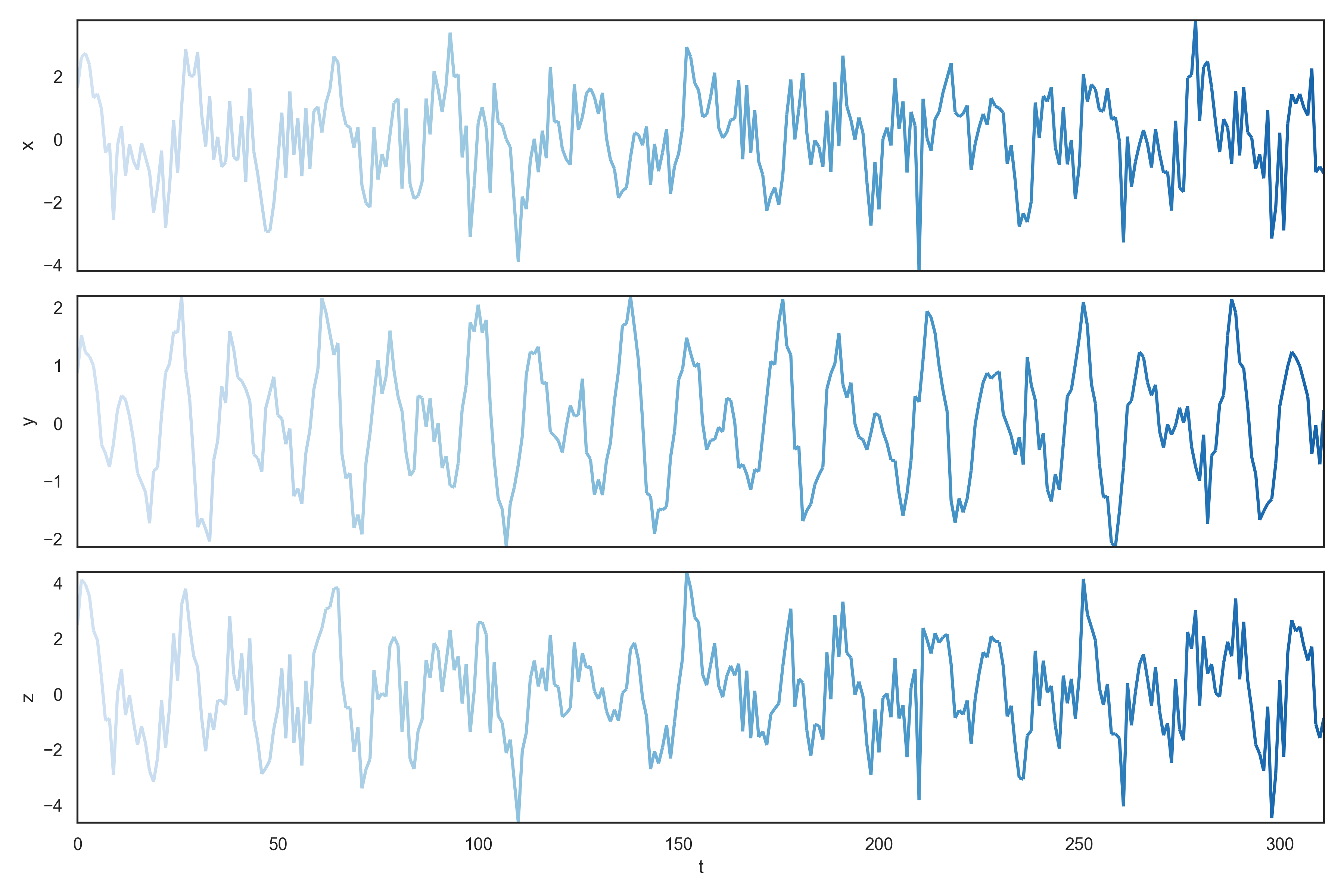
While nothing special appears when looking at the time series, the 3D trajectory quickly reveals the structure.
The hierarchy constrains the trajectory to the plane $z=x+y$ thus the system as whole only lives in 2 dimensions.
Hierarchical time series reconciliation
In order to visualize the necessity for hierarchical reconciliation, let us first forecast the 3 time series independently. We fit an ARIMA model on $x(t),y(t),z(t)$.
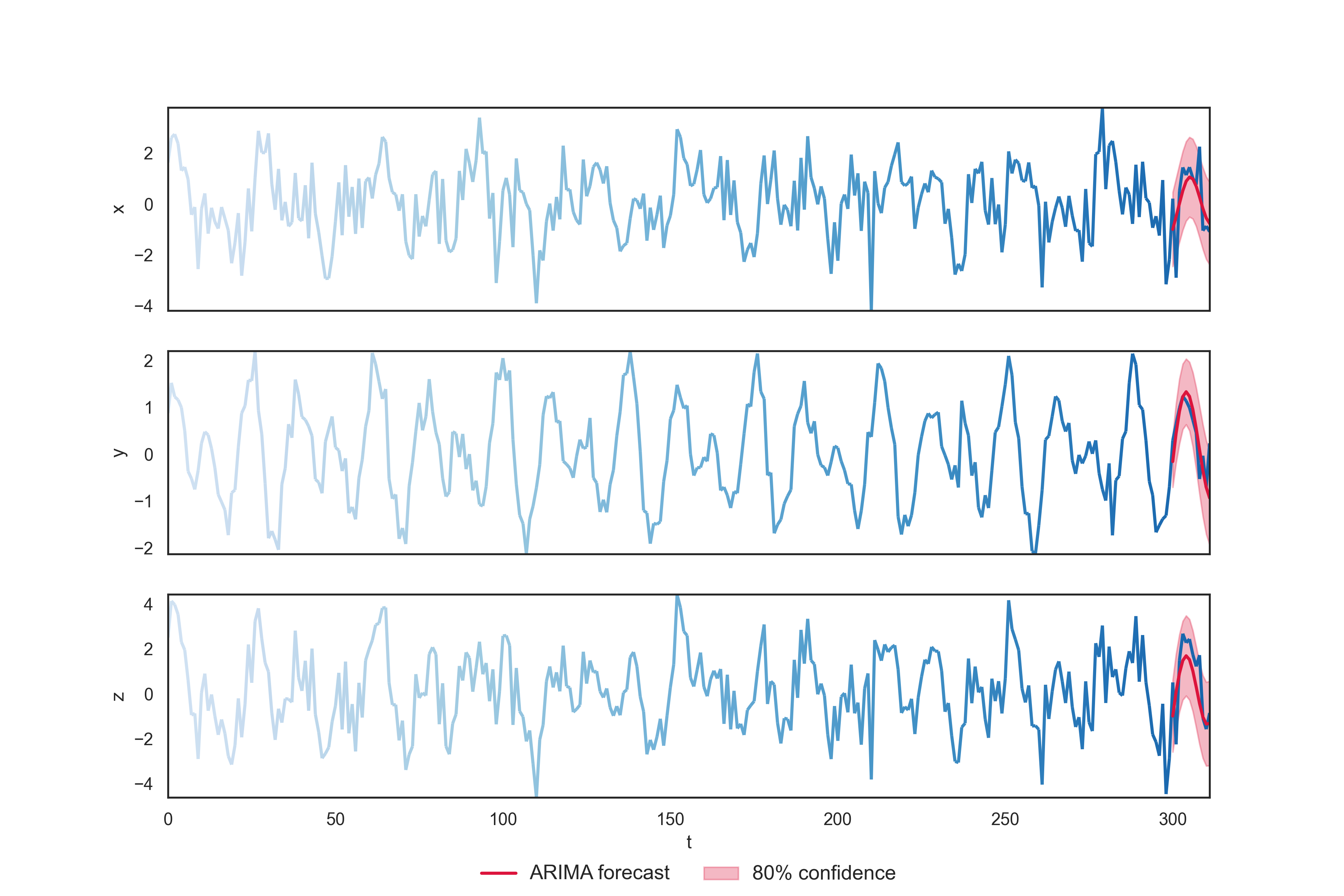
At first glance the forecast looks good, which is to be expected given the simple data we generated. However looking again at the trajectory, one can immediately view the incoherence. The ARIMA forecast is made of values the system cannot be in. Thus appears the reason why forecast reconciliation is useful, and often results in improvement in performance.
This interactive plot visually shows two of the most common hierarchical reconciliation methods namely Bottom-Up and GTOP or projection based reconciliation.
Bottom-Up consists in keeping the values of $x(t)$ and $y(t)$ fixed and setting $z(t) = x(t) + y(t)$. This is the simplest reconciliation method (one can observe that the reconciled forecast is lined up vertically with the original)
GTOP consists in projecting the forecast on the coherent plane. One can see the reconciled forecast is lined up with the original perpendicularly to the plane $z(t)=x(t)+y(t)$.